Working with native Excel tables

When you need to create certain types of content in your report template, it is often easier and more beneficial to use Microsoft Excel's native table features. This includes creating pivot tables, calculated columns, and calculated row totals.

It is recommended to convert your template content to native Excel tables if you want to do any of the following:

• Have easier access to native Excel data filtering and sorting

• Create a pivot table in your Excel report

• Add calculated columns which rely on native Excel computations

• Add calculated row totals which rely on native Excel computations

In some cases, you can accomplish these outcomes without converting content to native Excel tables. However, using this functionality is easier and is therefore the recommended workflow.

Creating native Excel pivot tables

A Qlik Sense pivot table can be added as a single table tag. You can recognize it from the add-in user interface because you cannot add it as individual columns. However, if you simply insert the Qlik Sense pivot table as a single-tag item with no other modifications, the chart will be exported as a straight table, not a native Excel pivot table.

Instead, complete the following steps to use Qlik Sense tabular data to create a native Excel pivot table:

1. Create or select a chart in your app to use as the source straight table. Insert it as a set of columns. See Adding content to your Excel report template.

2. Transform the chart table into a native Excel straight table.

3. Transform this native Excel straight table into a native Excel pivot table.

See below for details on each process.

Step 1: Insert the source data as a straight table

Design or select a chart in your Qlik Sense app with the columns you need to use to create the native Excel pivot table. This can be any Qlik Sense chart that has an underlying straight-table data structure (all supported visualizations except pivot table). If you are starting from scratch, a Table or Straight table (Visualization bundle) object might be the easiest input object to help visualize what you would like to add.

A native Excel pivot table performs aggregations on its own. Therefore, to include calculated expressions from the app in your Excel pivot table, add the non-aggregated fields from the Qlik Sense app as dimensions rather than measures.

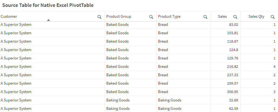
Next, add the chart to the report template as a set of individual columns. See Adding content to your Excel report template for instructions.

Step 2: Convert the tabular data to a native Excel straight table

When you have added the source Qlik Sense chart to the template, convert it to a native Excel straight table. Visit the Microsoft documentation for additional instructions. The following procedure is customized to provide details specific to your Qlik Excel template.

Do the following:

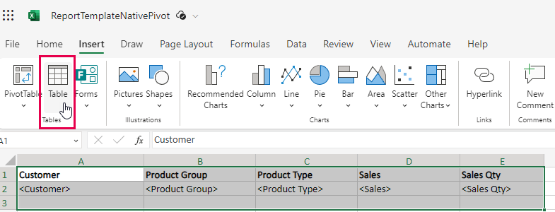
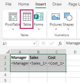
1. In Excel, highlight the area required to generate the native Excel table. This includes the header row, the row with tags, one additional row below these rows, and all desired columns. Convert the selection into a native Excel straight table.

   

2. With the native Excel straight table created, insert a <deleterow> tag below the row which has the column tags. This ensures the selected row is deleted in report output. For more information, see Removing rows with the Deleterow tag.

   

Step 3: Convert the native Excel straight table to a native Excel pivot table

Finally, transform the Excel straight table into an Excel PivotTable.

Visit the Microsoft documentation for additional instructions. The following procedure is customized to provide details specific to your Qlik Excel template.

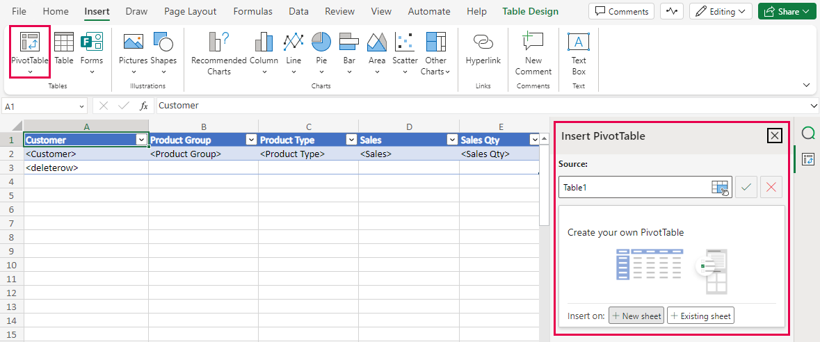
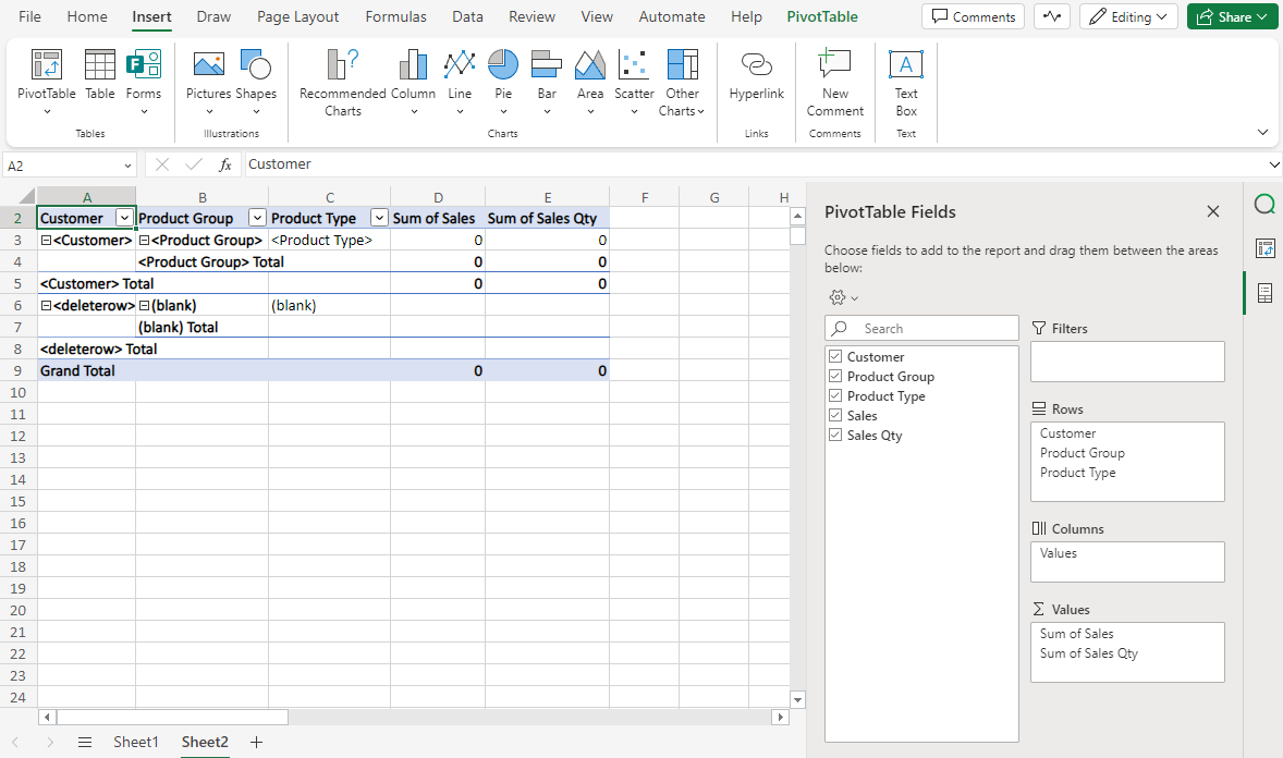
1. Select a cell within your native Excel straight table, and use the options in the Excel ribbon bar to convert it into a PivotTable.

   

2. Configure your pivot table with your desired configuration, using the Microsoft Excel features. If you need to have calculated expressions (measures) in your output, this is the step in which you would apply those aggregations.

   

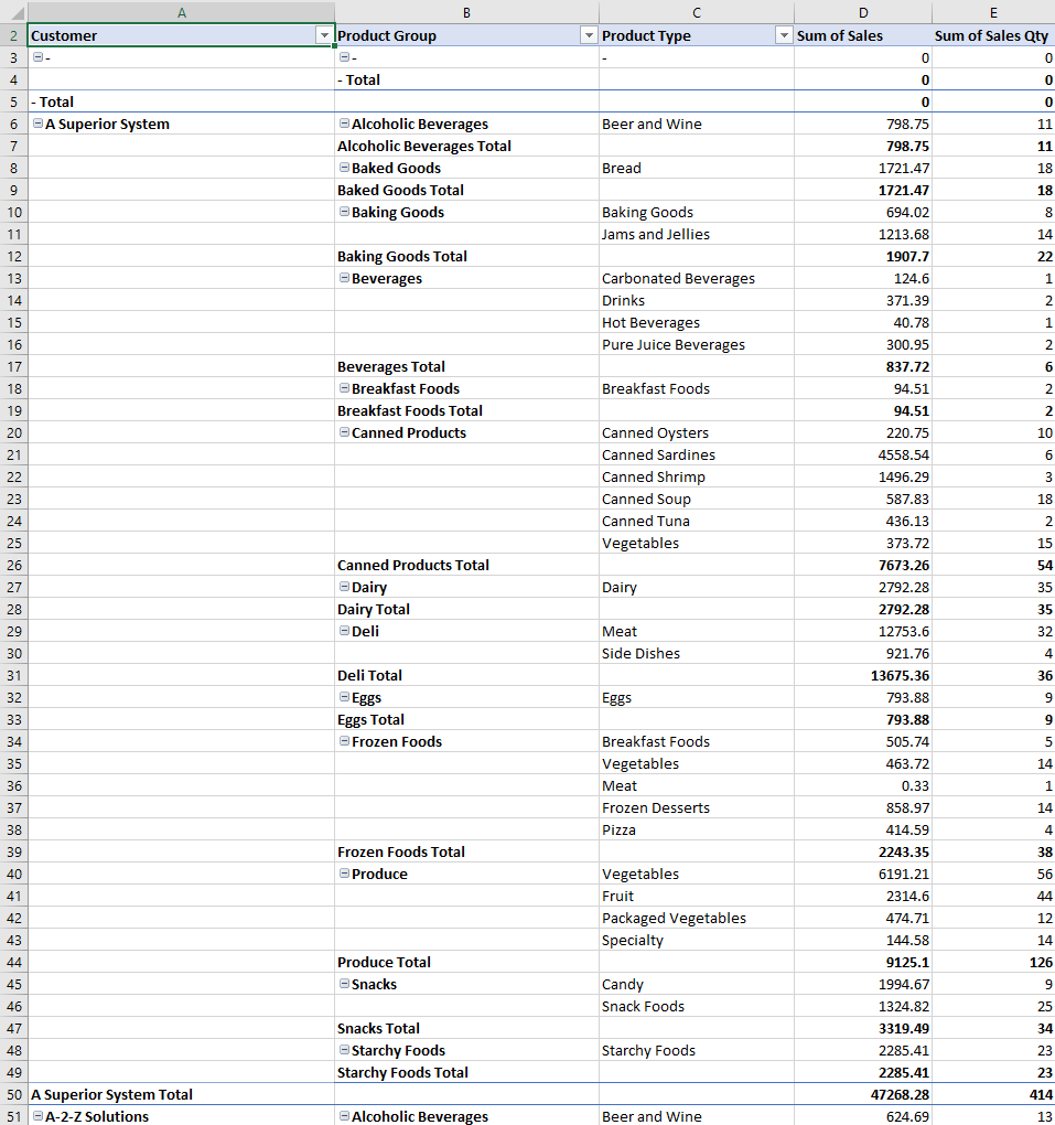
If you preview the report, the native Excel pivot table is generated correctly.

Adding calculated columns

You can use Excel formulas to add calculated columns that do not exist in your original Qlik Sense app. Use this functionality with both dimensions and measures defined in the source app.

Do the following:

1. Use the add-in to insert a Qlik Sense chart by column.

   

2. In Excel, highlight the area required to generate the native Excel table. This includes the header row, the row with tags, one additional row below these rows, and all desired columns. Convert the selection into a native Excel straight table.

   

3. To add a calculated column to the right of the rightmost column in your Excel table, click the cell to the right of the rightmost column tag, and type =, followed by your custom formula.

   

4. A new column is added to the Excel table. Note that it could have an invalid value in the template, but if configured correctly, it will generate the correct information in the output.

   You can rename the column, and format it as needed.

   

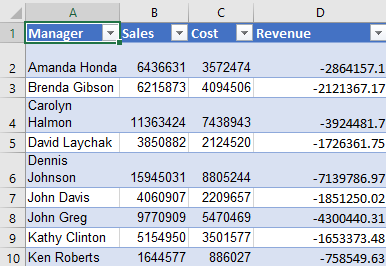
If you preview the report, you will see that the Excel table includes the new column, with the native formula being propagated in all rows.

Adding calculated totals

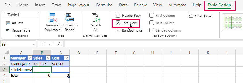
You can add a row that displays totals in your table by using native Excel features. Select the table, click on Table Design on the right, and select the Total Row checkbox.

Do the following:

1. Use the add-in to insert a Qlik Sense chart by column.

   

2. In Excel, highlight the area required to generate the native Excel table. This includes the header row, the row with tags, one additional row below these rows, and all desired columns. Convert the selection into a native Excel straight table.

   

3. With the native Excel straight table created, insert a <deleterow> tag below the row which has the column tags. This ensures the selected row is deleted in report output. For more information, see Removing rows with the Deleterow tag.

4. Click anywhere inside the table, and then click the Table Design tab in the Excel toolbar. Select the Total Row checkbox.

   

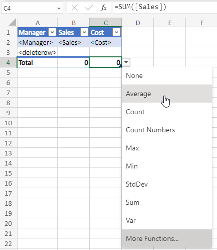
5. In the new Total row, click the cell for the column you want to have a total row for, and use the drop down to select any of the available built-in table summary functions.